
3D Reconstruction (2): Feature Tracks, Camera Registration, and Bundle Adjustment
Part one connected camera projection, epipolar constraints, and triangulation. Known cameras permit point recovery, while correspondences constrain camera motion. The eleven Castle images require both: features establish observations, tracks connect pairs into a scene, and bundle adjustment reconciles cameras and points under a common projection model.
We retain the world-to-camera convention \(\mathbf X_i=R_i\mathbf X+\mathbf t_i\). Observation \(\mathbf p_{ij}\) belongs to camera \(i\) and scene point \(j\). Only actual observed associations enter the objective.
1. Establishing local correspondences
Window ledges, doorway corners, and brick seams retain recognizable gradient layouts despite changes in image position, scale, and orientation. The Scale-Invariant Feature Transform (SIFT) searches scale space, assigns dominant orientation, and constructs a classic 128-dimensional local gradient descriptor. Detecting locations and describing appearance are related but distinct operations.
Scroll here to load the interactive figure.
Static preview / loading fallback
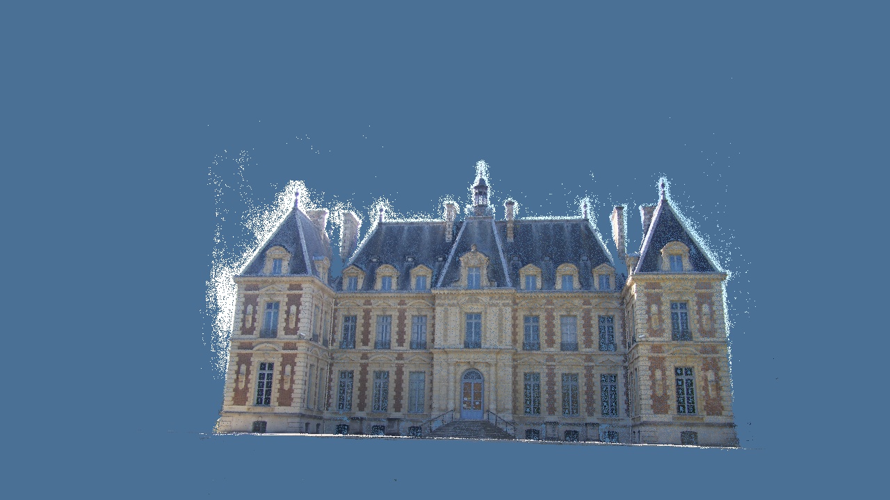
Select a frame or ledge and compare the crop centers. For a reference descriptor \(\mathbf f\), let \(d_1,d_2\) be its nearest and second-nearest support descriptor distances. The ratio test retains candidates satisfying
\[\frac{d_1}{d_2}<\tau\]The best match must stand out from an alternative, rather than merely have a modest absolute distance. Repeated panes can produce several similar descriptors, motivating this ambiguity check.
This widget extracts 2,500 features in each width 960 image, keeps 1,089 candidates at \(\tau=0.8\), then obtains 875 fundamental-matrix RANSAC inliers. Only a subset is drawn. It uses resized original images without prior undistortion, making its straight-line epipolar model approximate. Production geometry must handle observations under the correct camera model; part three’s independent plane sweep explicitly undistorts first.
Inliers still need scene interpretation. Repeated windows can support coherent mismatches, while planar facades may be explained by homography. Counts, coverage, parallax, and model type jointly determine suitability. These matches are independently computed teaching data, not upstream SfM tracks.
2. Tracks and new-camera registration
Pairwise correspondences must be associated across the collection. If a feature in A matches one in B, and that same B feature matches C, they may describe one three-view track. Write the track for point \(j\) as
\[\mathcal T_j=\{(i,\mathbf p_{ij})\mid i\in\mathcal V_j\}.\]Here \(\mathcal V_j\) is the set of images observing point \(j\). Conflicting positions within one image cannot be merged unconditionally. Stable, well-distributed tracks constrain multiple cameras; concentrated texture or moving foliage may provide weaker scene-wide support.
After initialization establishes some cameras and points, a new photograph can register through 2D–3D associations. Perspective-n-Point (PnP) estimates pose from existing \(\mathbf X_j\) and new-image \(\mathbf p_{ij}\). Its reprojection refinement can be written
\[(R_i^*,\mathbf t_i^*)= \arg\min_{R_i,\mathbf t_i} \sum_{j\in\mathcal J_i} \rho\!\left( \left\lVert\pi\!\left(K_i(R_i\mathbf X_j+\mathbf t_i)\right)-\mathbf p_{ij}\right\rVert^2 \right).\]The set \(\mathcal J_i\) contains valid new-image associations, \(\rho\) reduces outlier influence, and \(\pi((a,b,c)^\top)=(a/c,b/c)^\top\). Typically, robust sampling and a pose solver establish an initialization before nonlinear refinement.
PnP uses 2D–3D inputs, whereas initial relative pose uses 2D–2D correspondences. Registered images enable more triangulation and supply landmarks to subsequent images. The Castle run initializes eight views, adds three more, and repeatedly triangulates, filters, and refines this growing scene.
3. A joint reprojection objective
Separate pose estimation and triangulation produce an initial scene. Rotating one camera affects many projected points, while moving one point affects all cameras observing it. Bundle Adjustment (BA) places these dependencies into one optimization.
Let \(\mathbf c_i\) contain pose and selected intrinsics, with predicted pixel \(\hat{\mathbf p}_{ij}=\mathcal P(\mathbf c_i,\mathbf X_j)\). Define prediction-minus-observation residuals:
\[\mathbf r_{ij}=\mathcal P(\mathbf c_i,\mathbf X_j)-\mathbf p_{ij}.\]For valid observation set \(\Omega\) and image-coordinate covariance \(\Sigma_{ij}\), a common objective is
\[\min_{\{\mathbf c_i\},\{\mathbf X_j\}} \frac12\sum_{(i,j)\in\Omega} \rho\!\left(\mathbf r_{ij}^\top\Sigma_{ij}^{-1}\mathbf r_{ij}\right).\]Setting \(\Sigma_{ij}=I\) and \(\rho(s)=s\) yields ordinary squared reprojection distances. Covariance weights observation precision and direction; robust loss limits the dominance of unusually large discrepancies. These have different roles.
An incorrectly oriented Castle camera can distort many points to accommodate itself. Joint optimization uses other observations to constrain that compensation. A coherent repeated-window error may nevertheless evade robust loss, so verification and track management remain essential.
Derivation: Gaussian observations, whitened residuals, and robust loss
Independent zero-mean Gaussian image errors give likelihood terms proportional to
\[p(\mathbf p_{ij}\mid\mathbf c_i,\mathbf X_j) \propto \exp\!\left(-\frac12\mathbf r_{ij}^\top\Sigma_{ij}^{-1}\mathbf r_{ij}\right).\]Taking negative log-likelihood with fixed covariances yields weighted least squares. If \(L_{ij}^\top L_{ij}=\Sigma_{ij}^{-1}\), whitened residual \(\bar{\mathbf r}_{ij}=L_{ij}\mathbf r_{ij}\) has squared Euclidean norm equal to the original squared Mahalanobis distance.
Gross mismatches are not explained by that Gaussian model. One Huber loss on squared norm \(s\) is
\[\rho_\delta(s)= \begin{cases} s,&s\le\delta^2,\\ 2\delta\sqrt{s}-\delta^2,&s>\delta^2. \end{cases}\]Small discrepancies remain quadratic in distance; large ones grow more slowly. Threshold \(\delta\) must match the whitened error scale rather than being treated as unit-independent.
4. Local updates for a nonlinear objective
Depth division and constrained rotations make BA nonlinear. Locally parameterize all unknowns by \(\boldsymbol\theta\) and write
\[\mathbf r(\boldsymbol\theta\boxplus\Delta) \approx\mathbf r(\boldsymbol\theta)+J\Delta.\]The Jacobian \(J\) describes local sensitivity. The operator \(\boxplus\) applies an appropriate increment, particularly for rotation, instead of freely modifying matrix entries. With current local weights \(W\), a damped candidate update satisfies
\[(J^\top WJ+\lambda D)\Delta=-J^\top W\mathbf r.\]Positive diagonal scaling \(D\) and damping \(\lambda\) control step behavior. The solver evaluates actual improvement and adjusts how far to trust the local model. This is a fixed-weight local approximation, not a claim that every second-order robust-loss effect is captured by one constant \(W\). Levenberg–Marquardt and trust-region methods manage such approximations.
Derivation: perspective and pose-perturbation Jacobians
Ignoring distortion, let \(\mathbf X_i=(X_c,Y_c,Z_c)^\top\). Pixel derivatives with respect to camera coordinates are
\[J_{\rm proj}= \begin{pmatrix} f_x/Z_c&0&-f_xX_c/Z_c^2\\ 0&f_y/Z_c&-f_yY_c/Z_c^2 \end{pmatrix}.\]Thus the residual derivative with respect to a world point is \(J_{\mathbf X}=J_{\rm proj}R_i\).
Choose a small rigid perturbation applied on the left of the complete world-to-camera transform, ordered as \((\delta\mathbf v,\delta\boldsymbol\omega)\). To first order,
\[\mathbf X_i' \approx (I+[\delta\boldsymbol\omega]_\times)\mathbf X_i+\delta\mathbf v = \mathbf X_i+\delta\mathbf v-[\mathbf X_i]_\times\delta\boldsymbol\omega.\]Therefore
\[J_{\rm pose}= J_{\rm proj} \begin{bmatrix}I&-[\mathbf X_i]_\times\end{bmatrix}.\]The increment \(\delta\mathbf v\) belongs to that left rigid perturbation. It is not interchangeable with a parameterization that only adds to the original \(\mathbf t_i\). Right perturbations or another ordering require corresponding Jacobian changes.
Intrinsics, distortion, and whitening extend these derivatives through the chain rule. This ideal pinhole derivation provides a useful convention and sign check for implementations.
Scroll here to load the interactive figure.
Static preview / loading fallback
Blue dots are fixed noisy observations, orange crosses current predictions, and segments residuals. Four pinhole cameras observe eighteen points, giving 72 two-dimensional observations. Focal length and the first two poses are fixed; the other two poses and all points are optimized. Each observed image-coordinate component receives Gaussian noise with standard deviation 0.4 pixels.
The slider selects function-evaluation budgets from one shared initialization and displays actual solved snapshots. Global error falls from about 12.51 to 0.38 pixels using
\[{\rm RMS}= \sqrt{\frac1{\lvert\Omega\rvert} \sum_{(i,j)\in\Omega}\lVert\mathbf r_{ij}\rVert^2}.\]This is RMS of each observation’s 2D distance, not per-coordinate RMS or total solver cost. The experiment uses SciPy trust-region least squares to illustrate joint refinement. It is neither Castle BA history nor an iteration recording of Levenberg–Marquardt.
5. Exploiting bundle sparsity
An observation depends on one point, its camera, and possibly shared intrinsics rather than every scene point. Partitioning unknowns into camera and point increments gives
\[\begin{pmatrix}U&B\\B^\top&V\end{pmatrix} \begin{pmatrix}\Delta_c\\\Delta_x\end{pmatrix} = \begin{pmatrix}\mathbf b_c\\\mathbf b_x\end{pmatrix}.\]Without extra point-to-point priors, \(V\) consists of small point blocks. Eliminating point increments produces
\[(U-BV^{-1}B^\top)\Delta_c =\mathbf b_c-BV^{-1}\mathbf b_x.\]The Schur complement concentrates the solve on cameras while retaining their coupling through points. Point updates are recovered afterward.
Derivation: Schur elimination and point back-substitution
The second block row yields
\[B^\top\Delta_c+V\Delta_x=\mathbf b_x, \qquad \Delta_x=V^{-1}(\mathbf b_x-B^\top\Delta_c).\]Substitution into \(U\Delta_c+B\Delta_x=\mathbf b_c\) gives the reduced system. Implementations normally solve small systems to apply \(V^{-1}\) rather than forming a full inverse.
Shared calibration can sit on the camera side, while additional priors introduce residual blocks. Direct coupling between points changes the simple block-diagonal \(V\). Gauge constraints and suitable damping support stable local solves.
This structure also explains local versus global BA. A newly registered photo can trigger neighborhood refinement at lower cost, followed by broader optimization to reconcile accumulated discrepancies. Repeated Castle BA calls operate on changing observations and parameter confidence, not merely an identical fixed problem.
6. Gauge freedom and actual errors
Projection alone does not establish global translation, rotation, or uniform scale. For calibrated structure, transform all points by \(\mathbf X_j'=sQ\mathbf X_j+\mathbf a\), with positive scale \(s\), rotation \(Q\), and translation \(\mathbf a\). Matching camera changes preserve every image observation. These seven similarity freedoms are gauge freedoms.
Derivation: similarity invariance and gauge constraints
Choose
\[R_i'=R_iQ^\top, \qquad \mathbf t_i'=s\mathbf t_i-R_iQ^\top\mathbf a.\]Then
\[R_i'\mathbf X_j'+\mathbf t_i' =s(R_i\mathbf X_j+\mathbf t_i),\]Perspective obeys \(\pi(s\mathbf y)=\pi(\mathbf y)\), leaving reprojections unchanged. Fix a reference pose and constrain scale, or introduce known lengths, control points, or other priors. One fixed camera pose generally still leaves scale.
Fixing two complete poses in the teaching experiment provides a known baseline and is stronger than a universal minimum gauge constraint. Unknown calibration or degenerate motion can add ambiguity beyond these seven freedoms.
Intrinsics also need data-dependent treatment. Focal length, depth, and distortion can compensate for one another; freeing everything prematurely may let calibration absorb structural error. Shared lens models add constraints when justified, but zoom or other calibration changes may require grouping. Broad feature coverage and sufficient triangulation angles help distinguish effects.
One Castle initialization BA call uses eight images, 16,759 tracks, and 55,578 observations. Cost drops from about 52,361 to 12,532 before a reported mean error near 0.47 pixels. Later registration, refinement, and filtering yield a retained-observation mean near 0.44 pixels. Mean distance, the experiment’s RMS, and total cost are distinct statistics. They measure model agreement with retained observations, not complete-scene geometric accuracy.
7. Passing geometry to dense reconstruction
SfM supplies images, matching calibration, poses, and sparse structure in a common frame. Sparse points can inform neighbor selection and depth bounds. A PLY without cameras is generally insufficient for MVS; undistortion followed by resizing or cropping also requires consistent intrinsics.
The sparse stage now provides a shared geometric interpretation. Fixing cameras lets us estimate surface positions along more image rays. Part three develops plane-induced warps, real image costs, consistency, and fusion from that step.
Notation and references. \(\Omega\) is the observation set, \(\mathbf r_{ij}\) prediction-minus-observation residual, \(\Sigma_{ij}\) covariance, \(\rho\) robust loss, and \(J\) the local Jacobian. See the SIFT paper, Structure-from-Motion Revisited, and the Ceres tutorial and linear-solving documentation.
Data and reproduction. Castle photographs and logs come from the pinned OpenMVS sample, retaining its license. The matches and synthetic BA snapshots are independently generated; the latter contain no Castle poses or optimization history. Run python scripts/prepare_reconstruction.py with NumPy, SciPy, OpenCV, and Pillow to regenerate teaching data.
AI feedback
AnonymousLoading AI feedback…