
3D Reconstruction (3): Plane Sweeping, PatchMatch, and Multi-view Fusion
The previous article organized features into tracks and jointly refined cameras and sparse points. We now fix cameras and return to the brickwork around the doorway. Sparse landmarks support pose estimation, while many wall pixels still lack spatial locations. Multi-view Stereo (MVS) uses the same projection geometry to find evidence for those surface positions.
We follow reference-view depth and normal estimation followed by fusion. Relative projection leads to local-plane image warps, which are evaluated on real photographs. Plane sweeping, PatchMatch, and fusion then become connected stages of one estimation problem.
1. From a pixel to a local surface
Retain reference camera \(r\), support camera \(s\), and \(\mathbf X_s=R\mathbf X_r+\mathbf t\). The normalized ray is \(\mathbf q_r=K_r^{-1}\tilde{\mathbf p}_r\). At optical-axis depth \(Z\), its support projection is
\[\mathbf p_s(Z)= \pi\!\left(K_s\left(ZR\mathbf q_r+\mathbf t\right)\right).\]Varying \(Z\) moves this projection along the epipolar line derived in part one. Geometry restricts candidate positions; appearance helps select depth. These are reference-camera Z depths, requiring conversion if another system stores ray distances.
Individual colors are ambiguous, whereas frames and brick seams provide local structure. Approximate a neighborhood by a plane in reference-camera coordinates:
\[\mathbf n^\top\mathbf X_r=h, \qquad \lVert\mathbf n\rVert=1.\]Here \(\mathbf n\) is the normal and \(h\) signed plane offset. At the center, \(h=Z\mathbf n^\top\mathbf q_r\), so center depth plus normal defines the same local hypothesis. Projecting its entire reference neighborhood induces
\[\tilde{\mathbf p}_s\sim H_{sr}(\mathbf n,h)\tilde{\mathbf p}_r, \qquad H_{sr}=K_s\left(R+\frac{\mathbf t\mathbf n^\top}{h}\right)K_r^{-1}.\]The normal directly controls patch deformation. The front facade, side wing, and roof face different directions; translating window centers alone cannot generally align their texture. A local plane includes depth and orientation together.
Derivation: plane-induced homography and sign conventions
For every plane point, \(\mathbf n^\top\mathbf X_r=h\), hence
\[\mathbf t =\frac{\mathbf t\mathbf n^\top}{h}\mathbf X_r, \qquad \mathbf X_s= \left(R+\frac{\mathbf t\mathbf n^\top}{h}\right)\mathbf X_r.\]Substitute \(\mathbf X_r=Z_rK_r^{-1}\tilde{\mathbf p}_r\) and project into the support camera. Homogeneous scale removes \(Z_r\), yielding \(H_{sr}\).
If a source instead writes the plane as \(\mathbf n^\top\mathbf X_r+d_\pi=0\), then \(h=-d_\pi\) and its formula contains \(K_s(R-\mathbf t\mathbf n^\top/d_\pi)K_r^{-1}\). The sign difference follows the plane convention.
A neighboring ray intersects the plane at \(Z(\mathbf q)=h/(\mathbf n^\top\mathbf q)\). Near-zero denominators, negative depths, or invalid image projections do not provide suitable visible-surface samples. Also require \(h\ne0\): the plane cannot pass through the reference center.
2. Scoring geometric hypotheses in images
For \(N\) reference-window samples \(\mathbf p_k\), define intensities under one plane hypothesis as
\[a_k=I_r(\mathbf p_k), \qquad b_k=I_s\!\left(\pi(H_{sr}\tilde{\mathbf p}_k)\right).\]Warped coordinates are generally nonintegral, requiring interpolation. The experiment uses bilinear sampling and compares hypotheses on the same reference support, with normalization preserved across window sizes.
A direct Sum of Squared Differences (SSD) cost, averaged per sample and normalized by the 8-bit intensity range, is
\[C_{\rm SSD}=\frac1{N\,255^2}\sum_{k=1}^N(a_k-b_k)^2.\]Exposure affects this value even when geometry aligns. Zero-mean Normalized Cross-Correlation (ZNCC) removes each patch mean and normalizes variation:
\[{\rm ZNCC}= \frac{\sum_k(a_k-\bar a)(b_k-\bar b)} {\sqrt{\sum_k(a_k-\bar a)^2}\sqrt{\sum_k(b_k-\bar b)^2}}, \qquad C_{\rm NCC}=1-{\rm ZNCC}.\]With sufficient variation, \(C_{\rm NCC}\) ranges from zero to two, lower meaning more similar structure. Small denominators amplify noise, so weak texture requires a separate reliability decision.
Scroll here to load the interactive figure.
Static preview / loading fallback
Choose the doorway region and 21-pixel window, then move the candidate or jump to the minimum. The reference patch stays fixed while its support quadrilateral changes. Crops expose the local structure. The curve consists of actual evaluated costs rather than a drawn schematic.
The experiment undistorts two real photographs with the final logged calibration, independently estimates relative pose, and fixes \(\mathbf n=(0,0,1)^\top\). Thus \(h=Z\) and the implemented homography is \(K_s(R+\mathbf t\mathbf e_3^\top/Z)K_r^{-1}\). Translation has unit length, so depth is baseline-relative rather than meters or the full model’s display coordinates.
The 21-pixel doorway minimum is about 0.018 at relative depth 9.66. It is a good local appearance explanation under this pose, normal, and search range, not independently validated depth or a fused multi-view result.
Derivation: ZNCC invariance to global gain and offset
Transform the support patch by \(b_k'=\alpha b_k+\beta\), with \(\alpha>0\) and no clipping. Its mean is \(\bar b'=\alpha\bar b+\beta\), giving
\[b_k'-\bar b'=\alpha(b_k-\bar b).\]Both the correlation numerator and support norm gain the same factor \(\alpha\), which cancels. Thus \(\operatorname{ZNCC}(\mathbf a,\mathbf b')=\operatorname{ZNCC}(\mathbf a,\mathbf b)\). Negative gain would reverse correlation sign.
The experiment applies \(\alpha=1.2,\beta=20\) only during cost calculation and without clipping. SSD changes while ZNCC remains invariant. Shadows, saturation, reflections, and view-dependent highlights need not satisfy this patch-wide affine-intensity model.
Switching to repeated panes reveals competing local minima and window effects. Larger windows add context but may cross frame and background depths; smaller ones localize better but can lack distinctiveness. The sky’s 21-pixel reference standard deviation is only about \(0.70/255\). Its normalized curve still has a minimum, potentially dominated by tiny noise. The experiment preserves and flags that behavior; production systems combine texture, support, and consistency.
3. From plane sweeping to PatchMatch
The experiment evaluates 161 candidates uniformly in inverse depth \(\nu=1/Z\). Adjacent depth increments therefore differ. For rectified stereo, \(d=fB\nu\), so uniform inverse depth corresponds to uniform disparity and a useful image-space sampling resolution.
Searching depth and normal for every scene pixel makes exhaustive evaluation costly. PatchMatch exploits spatial coherence: a neighboring plane that explains brickwork is worth testing at the current pixel. Propagation transfers a plane, which must be intersected and rescored locally.
A neighboring plane \((\mathbf n_a,h_a)\) supplies current-pixel depth
\[Z_{\rm cand}(\mathbf p)= \frac{h_a}{\mathbf n_a^\top K_r^{-1}\tilde{\mathbf p}}.\]Two pixels on a slanted wall can have different depths while sharing that plane. Copying only a depth scalar loses this relationship. Random or progressively narrower perturbations explore hypotheses absent from the current neighborhood; reusable proposals still require acceptance based on observations.
Multi-scale processing passes broad estimates from lower resolution to finer refinement. Coarse support aids search but can merge narrow frames with background. Fine processing must retain opportunities to repair boundaries, and intrinsics must scale with each image. The widget performs fixed-normal two-view sweeping, not these full PatchMatch and scale operations.
4. Support views and geometric consistency
Additional photos add observations with different visibility. A doorway sidewall may be hidden while its upper edge remains visible. Image-level neighbors are commonly selected using shared landmarks, overlap, angle, and resolution, followed by local support decisions.
For support-image cost \(C_s(\mathbf p,Z,\mathbf n)\), one useful aggregation expression is
\[C_{\rm photo}=\sum_{s\in\mathcal S(\mathbf p)} w_sC_s(\mathbf p,Z,\mathbf n), \qquad w_s\ge0,\quad\sum_sw_s=1.\]This describes selected, weighted evidence rather than a universal implementation. Averaging all views admits occlusion contamination; selecting only the best view admits accidental repeated texture. Visibility, robust aggregation, and support count require joint treatment.
Appearance agreement alone is insufficient. When support view \(s\) has depth map \(D_s\), check whether it predicts the same spatial layer. A reference hypothesis projects with expected support depth
\[\mathbf X_s=R\!\left(Z_rK_r^{-1}\tilde{\mathbf p}_r\right)+\mathbf t, \qquad Z_s^{\rm pred}=\mathbf e_3^\top\mathbf X_s.\]Read valid \(D_s(\mathbf p_s)\), backproject, and transform back:
\[\mathbf X_r^{\rm back} =R^\top\!\left(D_s(\mathbf p_s)K_s^{-1}\tilde{\mathbf p}_s-\mathbf t\right), \qquad \mathbf p_r^{\rm back}=\pi(K_r\mathbf X_r^{\rm back}).\]Then evaluate round-trip pixel error and relative depth disagreement:
\[e_p=\lVert\mathbf p_r^{\rm back}-\mathbf p_r\rVert, \qquad e_Z=\frac{\lvert D_s(\mathbf p_s)-Z_s^{\rm pred}\rvert} {\max(D_s(\mathbf p_s),Z_s^{\rm pred})}.\]Use these on valid, positive-depth samples with meaningful visibility. A substantially nearer support depth can indicate an occluder; a farther measurement can indicate a free-space conflict. Invalid depth is not an ordinary zero-valued measurement.
Multiple views reduce some accidental matches, but their estimates share cameras, allowing systematic calibration errors to propagate. Thresholds depend on resolution, scale, and noise; fixed pixel tolerances do not imply fixed metric accuracy.
5. From depth observations to a common surface
Each depth map uses its own camera. A valid sample becomes world position
\[\mathbf X^{(i)}= R_i^\top\!\left(D_i(\mathbf p)K_i^{-1}\tilde{\mathbf p}-\mathbf t_i\right).\]Several reference images may measure the same window corner. Fusion first tests compatibility in position, depth, normal, and visibility, then aggregates. For measurements already identified as compatible, a simple weighted position is
\[\bar{\mathbf X}= \frac{\sum_i\omega_i\mathbf X^{(i)}}{\sum_i\omega_i}.\]Weights can reflect quality or support without implying statistical independence. Nearby foreground frames and recessed walls must not be merged indiscriminately. Stronger support thresholds reduce noise but may remove details visible in only a few images.
Scroll here to load the interactive figure.
Static preview / loading fallback
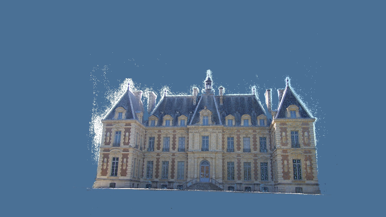
Switch points and mesh at a fixed view, then orbit slightly to inspect doorway and ledge layers. Point size changes display coverage rather than reconstruction completeness. Dense display sampling to 65,000 points also affects visible gaps. All 244,247 mesh triangles remain, without photographic texture concealing shape.
Upstream logs record eleven depth maps estimated at 1416×1064, producing 425,342 points after fusion and region trimming. Sample count minus fused-point count is not a direct surface-loss measure: multiple images observe the same surface and fusion includes filtering and deduplication.
6. Surfaces and reconstruction evaluation
Points record discrete measurements; meshes choose their connections. Methods use oriented samples, spatial partitions, visibility, or free-space evidence and differ in missing-region assumptions. Refinement can use images to adjust existing surfaces while remaining limited by topology and coverage. Subdivision does not establish an unseen rear surface.
Texturing separately handles image selection, exposure, seams, and atlases. A crisp brick seam may exist in color while geometry remains flat. Dimensional measurement therefore requires validation of the actual surface.
With independent references, accuracy concerns distances from reconstruction to reference surfaces; completeness concerns recovery of observable reference surfaces. Alignment scale, sampling, crop, and visibility conventions matter. This Castle viewer has no independent geometric ground truth, supporting qualitative inspection rather than millimeter claims or rankings. Reprojection fit, point counts, and visual appearance carry different evidence.
The series now closes its geometric chain: correspondences establish cameras and sparse points, BA reconciles observations, plane-induced projection supports dense matching with fixed cameras, and consistency and fusion organize a surface. Learned features and cost volumes change inference while retaining these geometric and visibility relationships.
7. Reproduction and further material
The preparation script converts complete upstream geometry and generates thumbnails, matches, synthetic BA, and the independent sweep. It does not rerun the entire Castle SfM/MVS pipeline. The sweep data record calibration, pose, and 161 inverse-depth candidates. Costs use uncompressed grayscale pixels, while displayed WebP photos have small compression differences.
Reproduction appendix: website data and the complete OpenMVS workflow
From the repository root, regenerate teaching data from pinned sources with NumPy, SciPy, OpenCV, and Pillow:
python scripts/prepare_reconstruction.py
Reconstructing all eleven original photos requires a separate OpenMVS installation containing CreateStructure and the full original images directory. This dense branch is extracted from the upstream script, omitting its sparse-mesh comparison:
CreateStructure -s images -o scene.sfm --export-mvs scene.mvs --extract-colors 1
DensifyPointCloud scene.mvs
ReconstructMesh scene_dense.mvs -p scene_dense.ply
RefineMesh scene_dense.mvs -m scene_dense_mesh.ply -o scene_dense_mesh_refine.mvs --scales 1 --max-face-area 16
TextureMesh scene_dense.mvs -m scene_dense_mesh_refine.ply -o scene_dense_mesh_refine_texture.mvs
Inspect cameras, depth intermediates, dense points, initial mesh, refined mesh, and textures in order. Retain versions, parameters, and logs. Resolution, support count, search range, and filtering affect both resources and point count; verify geometry before increasing detail.
Consult installed-version help. The full command chain was not run locally, and two webpage thumbnails cannot replace all original images. Other SfM formats require appropriate importers preserving images, calibration, and poses. See OpenMVS releases or the alternative COLMAP CLI pipeline.
Notation and references. \(Z\) is reference optical-axis depth, \(\nu=1/Z\) inverse depth, \((\mathbf n,h)\) describes \(\mathbf n^\top\mathbf X_r=h\), \(H_{sr}\) maps reference patches into the support image, and \(D_i\) is depth map \(i\). See PatchMatch Stereo, Pixelwise View Selection for Unstructured Multi-View Stereo, and the OpenMVS workflow.
Data and use. Complete interactive geometry comes from the pinned OpenMVS sample, not a new full reconstruction. The manifest records source counts and display transforms. The upstream AGPL-3.0 license is retained; material conditions follow the original source.
AI feedback
AnonymousLoading AI feedback…