
3D Reconstruction (1): Camera Projection, Epipolar Geometry, and Triangulation
This series uses eleven photographs of Sceaux Castle to review the geometry of recovering three-dimensional structure from images. We follow one chain of calculations: model projection, constrain camera motion with correspondences, recover spatial points, then extend observations into surfaces. Feature matching, Structure from Motion (SfM), bundle adjustment, and Multi-view Stereo (MVS) can then be understood in a shared geometric language.
Photographs and complete scene outputs come from the pinned official OpenMVS example. Essential definitions and results remain in the main narrative. Longer algebra is folded into optional derivations, so the case study remains readable with those sections closed.
1. From reconstruction back to image observations
Scroll here to load the interactive figure.
Static preview / loading fallback
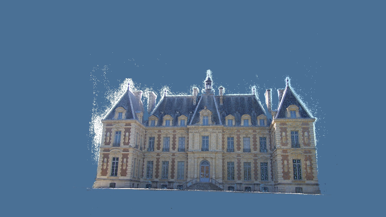
Switch stages in the frontal view: window frames and roof edges first appear as sparse landmarks, walls become denser, and triangles eventually organize a surface. A slight orbit reveals the depth of the central entrance and window ledges. Recovering these spatial relationships is the geometric task.
Let a fixed doorway detail be \(\mathbf X\), observed in image \(i\) at \(\mathbf p_i=(u_i,v_i)^\top\). Images supply these positions and local appearance; reconstruction must also recover calibration, camera poses, and spatial coordinates. One image collapses many locations along a viewing ray into one pixel. Multiple viewpoints constrain those possibilities jointly.
The upstream result contains 20,951 sparse points, 425,342 dense points, and 244,247 mesh triangles. The browser retains all sparse points and triangles, samples the dense cloud to 65,000 points, and applies a shared display transform. These counts describe representations, not measured accuracy.
2. Camera coordinates, perspective, and calibration
We use column vectors. A world point \(\mathbf X\in\mathbb R^3\) becomes a camera-coordinate point through
\[\mathbf X_i=R_i\mathbf X+\mathbf t_i, \qquad R_i\in SO(3).\]Here \(R_i\) is a rotation and \(\mathbf t_i\) belongs to the world-to-camera transformation. The world-space camera center satisfies \(R_i\mathbf C_i+\mathbf t_i=0\), giving
\[\mathbf C_i=-R_i^\top\mathbf t_i.\]This distinction matters when importing poses: the stored translation is not generally the camera’s world-space location.
For an undistorted pinhole image, define \(\tilde{\mathbf p}_i=(u_i,v_i,1)^\top\). Projection is
\[Z_i\tilde{\mathbf p}_i=K_i\mathbf X_i, \qquad K_i=\begin{pmatrix} f_{x,i}&0&c_{x,i}\\ 0&f_{y,i}&c_{y,i}\\ 0&0&1 \end{pmatrix}.\]This standard model assumes zero skew. Focal lengths \(f_x,f_y\) are measured in pixels, \((c_x,c_y)\) is the principal point, and \(Z_i\) is the third camera-coordinate component. Dividing by that component gives \(u=f_xX_i/Z_i+c_x\) and \(v=f_yY_i/Z_i+c_y\). Extrinsics establish camera coordinates; intrinsics map the resulting direction into pixels.
Conversely, \(\mathbf q_i=K_i^{-1}\tilde{\mathbf p}_i\) is a normalized viewing ray with third component one, so \(\mathbf X_i=Z_i\mathbf q_i\). The missing scalar is optical-axis depth. Euclidean distance along the ray is instead \(Z_i\lVert\mathbf q_i\rVert\).
Real lenses also distort images. Subsequent straight epipolar lines and matrix projections apply to corrected coordinates. Resizing by \(s_x,s_y\) requires \(K'=\operatorname{diag}(s_x,s_y,1)K\). The plane-sweep experiment handles both calibration scaling and distortion when converting width 2,832 photographs into width 960 images.
Derivation: homogeneous projection and relative camera transforms
With \(\tilde{\mathbf X}=(\mathbf X^\top,1)^\top\), projection becomes a \(3\times4\) matrix relation:
\[\tilde{\mathbf p}_i\sim P_i\tilde{\mathbf X}, \qquad P_i=K_i\begin{bmatrix}R_i&\mathbf t_i\end{bmatrix}.\]The symbol \(\sim\) means equality up to nonzero scale; a homogeneous vector is not yet a normalized pixel coordinate.
Using \(\mathbf X=R_r^\top(\mathbf X_r-\mathbf t_r)\) in the support camera gives
\[\begin{aligned} \mathbf X_s &=R_sR_r^\top\mathbf X_r+\mathbf t_s-R_sR_r^\top\mathbf t_r\\ &=R_{sr}\mathbf X_r+\mathbf t_{sr}, \end{aligned}\]Thus \(R_{sr}=R_sR_r^\top\) and \(\mathbf t_{sr}=\mathbf t_s-R_{sr}\mathbf t_r\). Throughout the series, subscript \(sr\) means a transformation from reference-camera coordinates \(r\) into support-camera coordinates \(s\).
For one image pair, abbreviate this as \(\mathbf X_s=R\mathbf X_r+\mathbf t\). Their projections then imply
\[Z_s\mathbf q_s=Z_rR\mathbf q_r+\mathbf t.\]This connects images, relative pose, and depth. Both epipolar geometry and plane sweeping will follow from it.
3. Disparity and depth scale
Consider parallel cameras, with the second center displaced rightward by baseline \(B\), identical focal length, rectified images, and equal horizontal principal points. Then \(R=I\) and \(\mathbf t=(-B,0,0)^\top\). A doorway point projects as
\[u_r=f\frac{X}{Z}+c_x, \qquad u_s=f\frac{X-B}{Z}+c_x.\]Subtracting gives disparity \(d=u_r-u_s=fB/Z\), hence
\[Z=\frac{fB}{d}.\]For a teaching configuration with focal length 1,200 pixels and baseline 0.5 meters, disparity 60 pixels means depth 10 meters. Measuring 61 pixels instead gives about 9.84 meters. At disparity 6 pixels, the same one-pixel discrepancy changes 100 meters to about 85.7 meters. These are illustrative numbers, not Castle metric calibration.
Differentiation expresses the sensitivity directly:
\[\frac{\partial Z}{\partial d}=-\frac{fB}{d^2}, \qquad \sigma_Z\approx\frac{Z^2}{fB}\,\sigma_d.\]The uncertainty approximation assumes known focal length and baseline and small disparity error. The same localization error produces greater depth uncertainty farther away. Larger baselines strengthen depth constraints but increase occlusion and appearance changes, so capture needs both overlapping neighbors and sufficiently distinct viewpoints.
This stereo arrangement is a special case. Arbitrary original images also contain rotation, unequal principal points, and distortion. Their raw horizontal displacements cannot be inserted directly into \(fB/d\); the general relative-projection relation must be retained.
4. Epipolar constraints from joint projection
In \(Z_s\mathbf q_s=Z_rR\mathbf q_r+\mathbf t\), vectors \(\mathbf q_s\), \(R\mathbf q_r\), and \(\mathbf t\) are coplanar. Eliminating depth through coplanarity yields
\[\mathbf q_s^\top E\mathbf q_r=0, \qquad E=[\mathbf t]_\times R.\]The skew-symmetric matrix obeys \([\mathbf t]_\times\mathbf a=\mathbf t\times\mathbf a\), and \(E\) is the essential matrix. Substituting \(\mathbf q=K^{-1}\tilde{\mathbf p}\) gives the pixel-coordinate form
\[\tilde{\mathbf p}_s^\top F\tilde{\mathbf p}_r=0, \qquad F=K_s^{-\top}EK_r^{-1}.\]The fundamental matrix \(F\) maps a fixed reference point to its support epipolar line, \(\boldsymbol\ell_s=F\tilde{\mathbf p}_r\). A true correspondence lies on that line, constraining a two-dimensional search to a one-dimensional locus. Other similar window corners can still lie along it, so appearance and robust estimation remain necessary.
Derivation: eliminating depth, epipoles, and essential-matrix structure
Set \(\mathbf a=R\mathbf q_r\) and take the inner product with \(\mathbf t\times\mathbf a\):
\[Z_s\mathbf q_s^\top(\mathbf t\times\mathbf a) =Z_r\mathbf a^\top(\mathbf t\times\mathbf a) +\mathbf t^\top(\mathbf t\times\mathbf a)=0.\]For nondegenerate finite visible points, this implies \(\mathbf q_s^\top[\mathbf t]_\times R\mathbf q_r=0\). Explicitly,
\[[\mathbf t]_\times= \begin{pmatrix} 0&-t_z&t_y\\ t_z&0&-t_x\\ -t_y&t_x&0 \end{pmatrix}.\]For nonzero translation, \(E\) has rank two and two equal nonzero singular values. Up to scale it has five effective degrees of freedom: three for rotation and two for translation direction. A rank-two homogeneous fundamental matrix has seven.
The reference camera center projects into the support image at epipole \(\tilde{\mathbf e}_s\sim K_s\mathbf t\). Since \(\mathbf t^\top[\mathbf t]_\times=0\), we have \(\tilde{\mathbf e}_s^\top F=0\). All support epipolar lines therefore pass through that epipole, which can lie outside the image or at infinity.
Under pure rotation, \(\mathbf t=0\), the essential matrix vanishes and provides no triangulation baseline. A nearly planar facade can also be strongly explained by a homography without reliably determining general 3D structure. Initialization needs useful parallax as well as model support.
5. From correspondences to relative pose
Appearance first proposes correspondences; geometric estimation fits \(F\) or \(E\) despite outliers. Unknown calibration often leads to fundamental-matrix estimation, while known calibration permits essential-matrix estimation in normalized coordinates. RANSAC samples small subsets and checks other observations, reducing the influence of wrong-window matches.
A common symmetric first-order approximation to geometric correspondence error is the Sampson error:
\[d_S^2= \frac{(\tilde{\mathbf p}_s^\top F\tilde{\mathbf p}_r)^2} {(F\tilde{\mathbf p}_r)_1^2+(F\tilde{\mathbf p}_r)_2^2 +(F^\top\tilde{\mathbf p}_s)_1^2+(F^\top\tilde{\mathbf p}_s)_2^2}.\]It normalizes the algebraic residual by local epipolar-line scale. Implementations can use different residual definitions and thresholds, so a “one-pixel” tolerance should not be transferred blindly between them.
Derivation: normalized eight-point estimation and pose decomposition
Flatten \(F\) row by row into \(\mathbf f\). Each correspondence gives
\[\begin{bmatrix} u_su_r&u_sv_r&u_s&v_su_r&v_sv_r&v_s&u_r&v_r&1 \end{bmatrix}\mathbf f=0.\]Stack at least eight nondegenerate correspondences into \(A\mathbf f=0\). With noise, minimizing \(\lVert A\mathbf f\rVert^2\) subject to \(\lVert\mathbf f\rVert=1\) selects the right singular vector associated with the smallest singular value. Translating and scaling image coordinates improves conditioning. If the normalizations are \(T_r,T_s\), undo them with \(F=T_s^\top F_nT_r\).
Enforce rank two by zeroing the smallest singular value. With calibration, form \(E=K_s^\top FK_r\) and project its singular values to \((a,a,0)\), where \(a\) averages the first two. This explains a basic linear route; calibrated minimal solvers can estimate \(E\) from fewer correspondences.
Let \(E=U\operatorname{diag}(a,a,0)V^\top\), adjusting signs so candidate rotations have determinant one, and define
\[W=\begin{pmatrix}0&-1&0\\1&0&0\\0&0&1\end{pmatrix}.\]Rotations are \(UWV^\top\) and \(UW^\top V^\top\), paired with translation directions \(\pm U_{:,3}\). Triangulate reliable correspondences for the four combinations and select one supporting sufficiently many points in front of both cameras. Translation magnitude remains unknown and is commonly normalized to one.
Relative pose now puts viewing rays into a shared frame. Without a length reference, scene and baseline can be scaled together without altering projection. Part three uses unit-baseline depth; the complete model has a separate display normalization. Neither automatically supplies meters.
6. Triangulation and reprojection
With known projection matrices, \(\tilde{\mathbf p}_i\sim P_i\tilde{\mathbf X}\) implies \([\tilde{\mathbf p}_i]_\times P_i\tilde{\mathbf X}=0\). Two independent constraints per view provide a linear homogeneous point estimate.
For a Castle corner, this finds a location compatible with its viewing rays. Noise prevents exact ray intersection. After linear initialization, refine the point by minimizing image reprojection error:
\[\mathbf X^*=\arg\min_{\mathbf X} \sum_i\left\lVert \pi\!\left(K_i(R_i\mathbf X+\mathbf t_i)\right)-\mathbf p_i \right\rVert^2, \qquad \pi\begin{pmatrix}a\\b\\c\end{pmatrix}= \begin{pmatrix}a/c\\b/c\end{pmatrix}.\]This measures discrepancy in observation space rather than algebraic equation residuals. Allowing camera parameters to change turns it naturally into the joint adjustment developed next.
Derivation: linear triangulation and positive-depth checks
Write the three rows of \(P_i\) as \(\mathbf a_{i1}^\top,\mathbf a_{i2}^\top,\mathbf a_{i3}^\top\). Eliminating projective scale gives
\[(u_i\mathbf a_{i3}^\top-\mathbf a_{i1}^\top)\tilde{\mathbf X}=0, \qquad (v_i\mathbf a_{i3}^\top-\mathbf a_{i2}^\top)\tilde{\mathbf X}=0.\]Stack these rows into \(A\) and take its smallest-singular-value right vector. Divide by the last homogeneous component when nonzero; a near-zero component suggests a distant point rather than stable finite structure.
Check \(Z_i=\mathbf e_3^\top(R_i\mathbf X+\mathbf t_i)>0\), reprojection error, and ray angle. Positive depth only places the point in front of the camera. Nearly parallel rays can still give uncertain depth despite a low current reprojection error.
The world-space ray from camera center has direction \(R_i^\top\mathbf q_i\). When ray angles are small, slight image perturbations move their intersection substantially. This is consistent with the stereo uncertainty relation and motivates parallax checks during initialization and point filtering.
7. From two views to the Castle scene
One doorway detail has now connected camera projection, epipolar constraints, and triangulation. More photos require tracks, registration into existing structure, and joint refinement. These operations form SfM and supply camera geometry to MVS.
The upstream log records eleven poses, one shared intrinsic model, 249,509 features, and 55 pairs. Shared intrinsics do not mean one viewpoint. This run initializes eight views, registers three more, and interleaves triangulation, filtering, and optimization before exporting 20,951 sparse points. Particular initialization strategies vary, while the geometric quantities remain the same.
Part two follows actual correspondences into PnP and bundle adjustment. Part three returns to relative projection to derive plane-induced image warps and dense matching.
Notation and references. \(\mathbf X\) is a world point; \(R_i,\mathbf t_i\) transform world to camera; \(K_i\) is calibration; \(\mathbf q_i\) is a normalized ray; \(Z_i\) is optical-axis depth; \(B\) is baseline and \(d\) rectified disparity. See Hartley and Zisserman’s Multiple View Geometry and the OpenCV calibration documentation for further material and interfaces. Derivations here follow the stated conventions; other conventions require corresponding sign and transform changes.
Data and sources. Complete geometry is a pinned upstream output, not a full SfM/MVS rerun. The manifest records hashes, counts, and display transforms; prepare_reconstruction.py performs conversion. The upstream AGPL-3.0 license is retained; consult the original source for individual material conditions.
AI feedback
AnonymousLoading AI feedback…