中文版

• Nyquist–Shannon sampling theorem
  • Fourier-Transform
  • Convolution
  • Aliasing
  • Sampling Theorem
  • Filtering

Introduction: Anti-aliasing is a long-standing topic in the field of graphics rendering. Due to the limited resolution of display devices and the demand for high-resolution textures in applications, the aliasing problem is one that frequently arises in graphical applications.

The impact of aliasing on visual effects is significant, and various anti-aliasing methods have been developed to address it, each based on different causes. Based on my practical work experience, I have provided a brief summary of common anti-aliasing algorithms.

Readers are welcome to discuss and share their insights, and any corrections or suggestions are appreciated.

Since the aliasing issue is essentially a problem of aliasing in signal processing, this article begins with a brief review of sampling theory.

Nyquist–Shannon sampling theoremPermalink

Fourier-TransformPermalink

In the physical world, signals are generally continuous, represented as $s(t)$. In signal processing systems, analyzing the frequency components of the input signal (frequency spectrum analysis) is typically very important. This is usually done by applying the Fourier Transform to convert the signal from the time domain to the frequency domain. The formula for the Fourier Transform is as follows.

[Wikipedia Fourier-Transform]

Common functions in signal systems and their Fourier Transforms are as follows:

Time-domain function	Frequency-domain function	Illustration	Description
Impulse	Constant		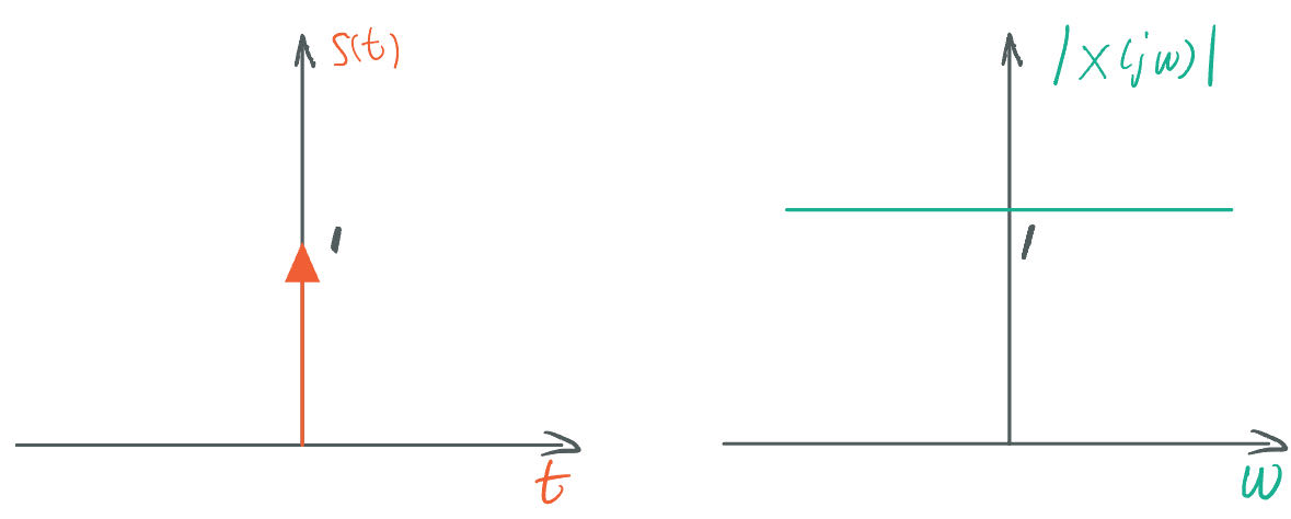The impulse function at the origin and the constant function are mutual Fourier Transforms. The Fourier Transform of an impulse function not at the origin is a linear function.
Dirac Comb	Dirac Comb		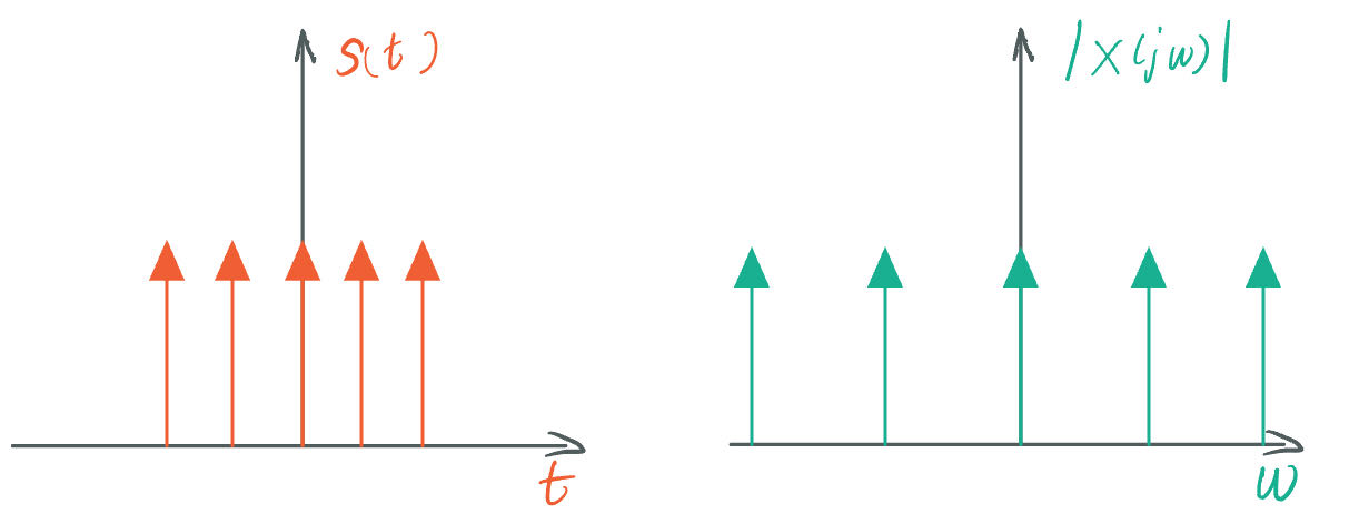The Fourier Transform of a Dirac comb function is also a Dirac comb function, with their spacing inversely proportional to each other.
Rect Window	Sinc		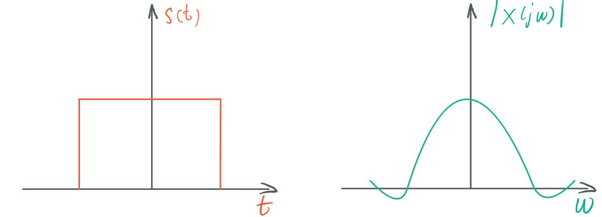The rectangular window function and the Sinc function are mutual Fourier Transforms.
Gaussian	Gaussian		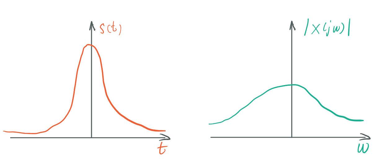The Fourier Transform of a Gaussian function is also a Gaussian function, with their variances being inversely proportional to each other.

ConvolutionPermalink

Convolution is a type of operation between two signals, commonly used in frequency spectrum analysis of signal systems. The convolution operation between two signals is given by the following formula. [Wikipedia Convolution]

Some important properties are as follows:

• Multiplying two functions in the time domain is equivalent to convolving the two functions in the frequency domain, and vice versa.
• Convolution of a function with an impulse function (whether at the origin or not) is equivalent to reconstructing the function at the position of the impulse (considering the amplitude of the impulse).
• Convolution operation has linear properties, satisfying commutativity and associativity. Therefore, convolution of an input function with a comb function is equivalent to the sum of the convolution results of the input function with each impulse component of the comb function.
• The Fourier Transform of a comb function is still a comb function, with the spacing of the comb function in the time domain being inversely proportional to the spacing of the corresponding comb function in the frequency domain.
• Convolution of two Gaussian functions is still a Gaussian function, with the resulting variance being the sum of the variances of the two input Gaussians.
• The frequency spectrum function is symmetric about the origin, which is a fairly intuitive conclusion.

Convolution of a function with an impulse function in the time domain is equivalent to multiplying their Fourier Transforms in the frequency domain. Since the frequency spectrum of an impulse function is a linear function, the final result is essentially the reconstruction of the input function at the position of the impulse.

The above properties can all be proven through Fourier Transform and convolution operations.

AliasingPermalink

For a time signal system $s(t)$, the sampling operation typically involves sampling the original signal at regular intervals (sampling intervals), resulting in a discrete set of values. These discrete values are then used to reconstruct the original signal. This process is equivalent to multiplying the original signal $s(t)$ with a sampling comb function $f(t)$, as illustrated in the following diagram.

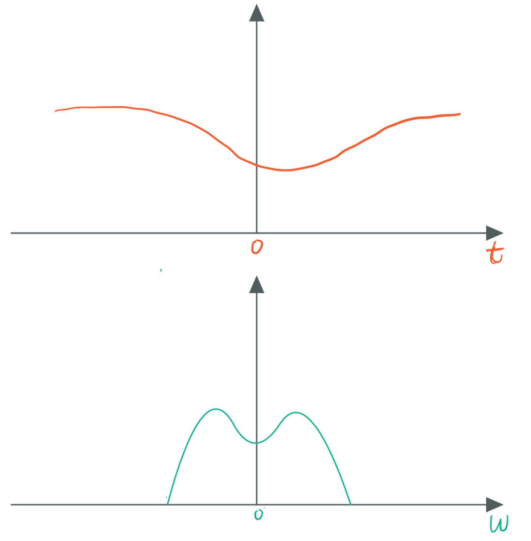
This is equivalent to convolving the frequency spectrum function $S(\omega )$ of the original signal with the frequency spectrum function $F(\omega )$ of the comb function, as illustrated in the following diagram.

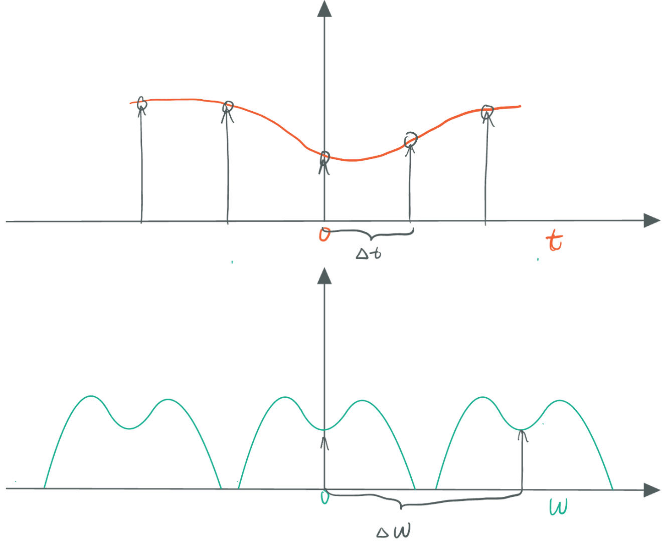
Since the Fourier Transform of a comb function is still a comb function, the convolution result in the frequency domain is as shown in the diagram. In this case, there is no aliasing, and the frequency spectrum functions do not overlap.

We know that the frequency spectrum function of the input signal is symmetric, with a maximum frequency of ${\omega }_{max}$​. When $\mathrm{\Delta }\omega <2\ast {\omega }_{max}$​, the frequency spectrum functions will overlap, leading to aliasing. Aliasing causes the sampled values to be insufficient for accurately reconstructing the original function in the time domain, resulting in distortion.

The original function discussed is a function of time tt. When the original function is a function of spatial coordinates, aliasing can also cause distortion in space.

Whether sampling in the time dimension or the spatial dimension, aliasing effects can result in noticeable visual distortions. Common examples include:

• Observing a car wheel spinning rapidly, where the wheel may appear to be “reversing” (time dimension).
• Taking a photograph of a display screen with a phone, which can produce moiré patterns (spatial dimension).

Sampling TheoremPermalink

Based on the above conclusions, to avoid distortion, it is necessary to satisfy $\mathrm{\Delta }\omega >2\ast {\omega }_{max}$. This means the sampling frequency must be greater than twice the highest frequency in the original signal to ensure that the convolution in the frequency domain does not result in function overlap, thereby avoiding aliasing.

The sampling theorem is quite simple. For existing aliasing issues, all remedial actions revolve around the sampling theorem and can be categorized into two approaches:

1. Apply low-pass filtering to the original function to remove high-frequency components.
2. Increase the sampling frequency to meet the requirements of the sampling theorem.

FilteringPermalink

Suppose the original signal function is $s(t)$ and the filter function is $g(t)$. The filtering operation is the convolution of $s(t)$ and $g(t)$, which, in the frequency domain, corresponds to multiplying their Fourier Transforms. To filter out high-frequency information from the original signal, the ideal low-pass filter in the frequency domain would be represented by a window function. However, a window function in the frequency domain translates to an irregular filter kernel in the time domain, which increases computational complexity.

We can evaluate filter functions based on their characteristics. Examples of time-domain filter functions include:

• Rectangular Window Function: Simple to compute and performs weighted averaging, but it can miss high-frequency information in the frequency domain, resulting in poor filtering quality.
• Gaussian Function: Requires a significant size for the Gaussian kernel, which makes it computationally intensive, but it provides a better frequency response.
• Other Window Functions: Such as Rectangular Window, Hanning Window, Hamming Window, and Blackman Window. [Wikipedia Window Function]

The content of this blog post is original to the author. Please indicate the source and include the original link when reproducing it. Thank you for your support and understanding.